Difference between revisions of "YOLO algorithm"
(begin yolo v7 model section) |
m (end the horrible wrapping between two images) |
||
| Line 3: | Line 3: | ||
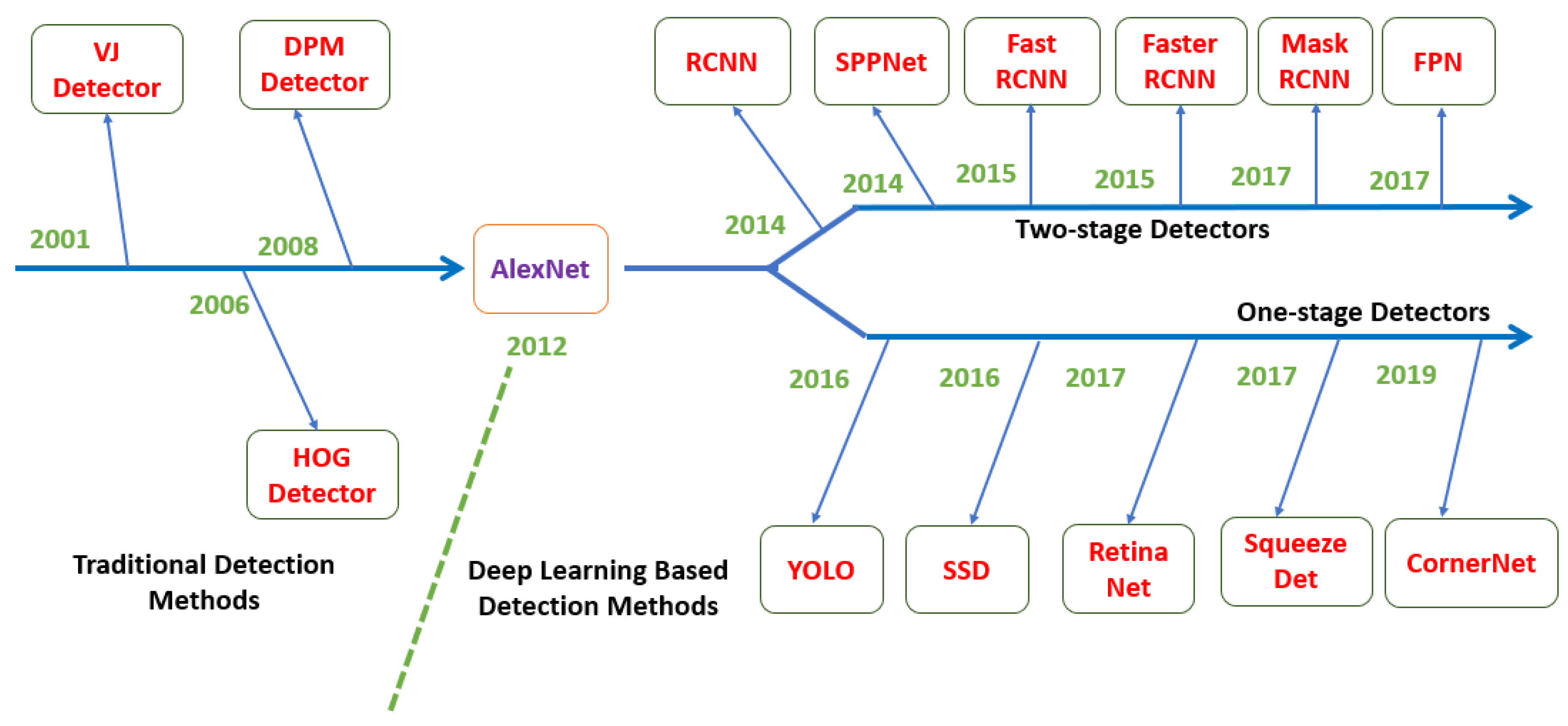
[[File:Timeline.png|thumb|490px|left|YOLO was the first first-look object detection algorithm and has given rise to a whole class of modern detection algorithms]] | [[File:Timeline.png|thumb|490px|left|YOLO was the first first-look object detection algorithm and has given rise to a whole class of modern detection algorithms]] | ||
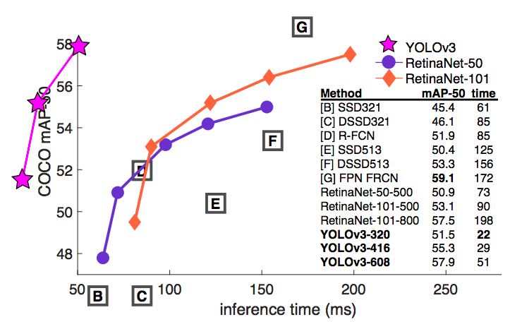
| − | [[File:Performance.png|thumb|485px| | + | [[File:Performance.png|thumb|485px|center|YOLO performance as compared to state-of-the-art at the time of publication]] |
| − | + | ||
==How Does YOLO Work?== | ==How Does YOLO Work?== | ||
Revision as of 19:29, 13 December 2022
Contents
What is YOLO and why is it so revolutionary?
YOLO (you only look once) is a real-time object detection algorithm originally proposed in Redmon et al. 2016. One of the ways the YOLO algorithm revolutionized the field of object-detection is that it was the first algorithm that implemented a 1-look approach to object detection. In the case of multi class object detection, instead of running an algorithm once for each class, YOLO performs a single pass over the image and generates all of the bounding boxes for detected objects. The ability to produce predictions after a single pass over the image allowed YOLO to be much faster than other state-of-the-art algorithms in 2016. While the original YOLO algorithm performed slightly below other object detection algorithms of the time, the drastic improvement in inference time made it suitable for real-time applications. Below are a timeline showing how YOLO gave rise to the class of one-look algorithms (left) and a plot showing YOLO's performance and inference time plotted against other state-of-the-art algorithms at the time (right).
How Does YOLO Work?
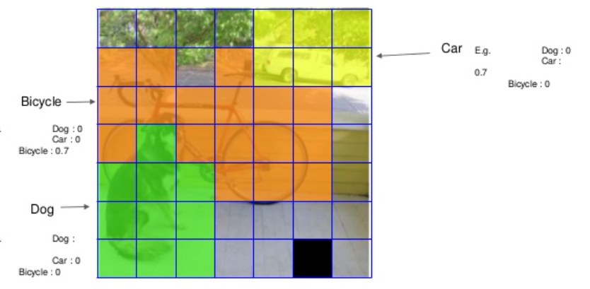
The YOLO algorithm begins by taking in an image as input. It then divides the image in to squares of size S by S pixels. The algorithm's job is to predict which of these cells contains the center of an object, and if it does, a probability distribution over the C classes it is trying to predict. In order to make these predictions, the original YOLO v1 model used a convolutional neural network made up of 24 convolutional layers and max suppression layers followed by fully connected layers. Each of these cells makes B predictions for where an object is in the cell. Each of these predictions is called a bounding box. For each of the cells, the algorithm outputs B prediction vectors. Each of these vectors is made up of 6 parts and appears as such: [p, x, y, h, w, c] where p is the probability of an object being in the box, x and y are the center of the object, h and w are the height and width of the object, and c is a one-hot encoded vector representing the C classes. Everything in this section so far makes up the YOLO algorithm. It took as input an image, and returned B vectors for each of the cells it divided the picture into at the beginning. At this point, we have B predicted objects, but it turns out that this is usually far too many and that many of these boxes are not actually of objects or multiple end up being of the same object. In order to remove the boxes that are not likely to be of objects, a two stage approach is taken. Firstly, any box that has a low certainty of an object being in it is removed. This removes boxes that were not likely to have had objects. Next max suppression is used to remove duplicate boxes that are detecting the same image. In max suppression, boxes with the same predicted class are removed if there is one that is a better fit to the ground truth label. This measure of being a better fit is known as IoU (Intersection over Union) where a box's score is the area of intersection between the predicted box and the true box divided by the union of their areas. After this two step filter, we are left with only images that have a relatively high confidence and images that are of distinct objects.
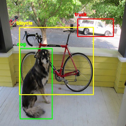
Here are some images that point out some of the key concepts about how the YOLO algorithm detects objects. Left: Each image is divided into cells and a single prediction is made per cell after taking the best bounding box per cell. Right: Shows how once the best boxes are shown, that there are far too many and how after the 2 stage filtering, only the high confidence distinct boxes remain.
Sample Inferences
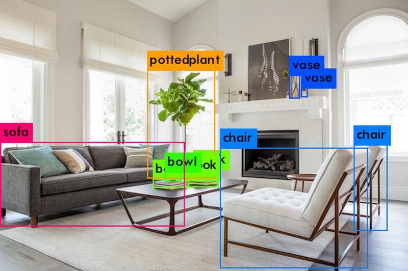
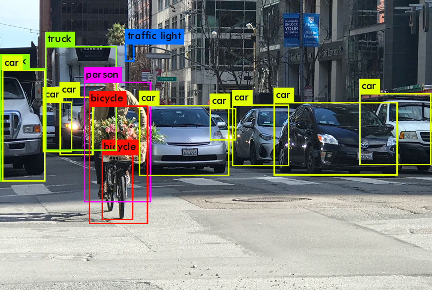
The most typical set that YOLO is trained on is the Common Objects in Context (COCO) dataset. The COCO dataset originally had 80 classes of objects and has been adding more as they expand the dataset. The YOLO algorithm takes in an image and returns bounding boxes around each of the instances detected. Here are some samples.
YOLO V4 Model
The repository for our current model is hosted on the Autobike Github. These instructions essentially detail how we made that model, and then how to re-train, run, test, and demo it.
Preparing Data
First, we download the COCO 2017 dataset - we want train, test, and validation images. Note that during our training in Fall 2021, we did not use test data, so I'll just be mentioning train and validation images.
Search through the download to find the annotation files - they should be called instances_train2017.json and instances_val2017.json. Additionally, you'll want to make sure you know the file path to each set of images.
Now is a good time to move around the image folders to a more permanent location - it doesn't matter where they are, as long as you have the file path.
In the coco_annotation.py file in the scripts folder, plug the file path for the annotations into json_file_path and the images into images_dir_path. As with all the scripts we run,
you'll need to run it once for each set of images you have. You've now got a Darknet version of the COCO annotations, but we haven't filtered the images at all.
To filter the images, we'll delete any annotation that doesn't contain one of the categories we want. This script is called remove_unecessary_cats.py. You can see at the top of the file we have a dictionary with all of our
desired categories. These IDs are pulled from the COCO dataset (more specifically, sites online that list all the categories in order).
objectIDs = {
    1:'person',
    2:'bicycle',
    3:'car',
    4:'motorcycle',
    6:'bus',
    8:'truck',
    10:'traffic light',
    11:'fire hydrant',
    13:'stop sign',
    14:'parking meter',
    15:'bench',
    17:'cat',
    18:'dog',
    64:'potted plant'
}
Run the annotation files through this script.
This is good, but now the category numbers are wrong - potted plant isn't the 64th category anymore. We specify the categories in a
file called coco.names, under data. We fix the categories by running the annotations through match.py,
also in the scripts folder.
Finally, we need to create an annotation file for each useful image, instead of one condensed annotation file. We can do this automatically by once again
running our annotations through a script, convert_annotations.py. Take note of where your final train.txt file ends up.
We tell the model where all of our information is in a file called coco.data in the data folder.
classes = 14
train  = data/train.txt
valid  = data/val.txt
names = data/coco.names
backup = backup
We've put our train, val, and names files in the data folder. We also have 14 classes, as specificed above. The backup folder is going to hold mid- and post-run weights to save the model state.
Configuring the Model
The majority of this section is derived from the 'How to train (to detect your custom objects)' section of the Darknet README.
First, download this weights file, called yolov4.conv.137, which will serve as our starting point from which to train the model.
Next, copy the yolov4-custom.cfg file, and rename it to yolo-obj.cfg. Then, follow these steps to adjust the model.
- Change batch to
batch=64 - Change subdivisions to
subdivisions=16(this may need to be adjusted depending on your computer's architecture) - Change max batches to
classes * 2000, but not fewer than the number of training images (so for our model, we did 90,000) - Change steps to 80%, 90% of
max_batches - Set network size to
width=416andheight=416or any multiple of 32 - Change
classes=80to our class number in each of 3 [yolo]-layers - Change
filters=255tofilters=(classes+5)*3in the 3 [convolutional] layers before each [yolo] layer (and ONLY the [convolutional] directly before [yolo])
For reference, you can check out our current yolo-obj.cfg file on the Github.
Commands
Train the model using your coco.data file from preparing the data, and yolo-obj.cfg, yolov4.conv.137 from configuring the model.
./darknet detector train data/coco.data cfg/yolo-obj.cfg yolov4.conv.137
Sample test the model's prediction on individual images using this interactive command:
./darknet detector test data/coco.data cfg/yolo-obj.cfg backup/yolo-obj_final.weights
where coco.data and yolo-obj.cfg are the files you trained on.
The yolo-obj_final.weights file is automatically generated if the model completes its full training run, but you can use any other *.weights file you'd like.
Get specific validation statistics for the model using this command:
./darknet detector valid data/coco.data cfg/yolo-obj.cfg backup/yolo-obj_final.weights
The three files referenced mimic the usage in the test command.
Run the model on a video input using this command:
./darknet detector demo data/coco.data cfg/yolo-obj.cfg backup/yolo-obj_final.weights -ext_output /home/autobike/Downloads/trafficvideo.mp4
The first three files mimic the usage in the test and validation commands. The -ext_output flag allows you to specify the video - here, we're running it on trafficvideo.mp4 in the Downloads folder.
YOLO V7 Model
In Fall 2022, we were able to run the (at the time) newest version of the model available. We heavily referenced this tutorial which explains how to deploy this model to the Jetson Nano on a dataset made up of pothole images. We first got it to work using those images, then switched over to the full COCO dataset (not the reduced set explained above, due to time constraints).
